We assume that cells (or transcripts) can be approximated as points locations.
spatstat package and ppp object
A powerful package to analyse point patterns in R is called spatstat(Baddeley and Turner 2005). The main data object to compute on is called a ppp object. ppp objects describe point patterns in two dimensional space, ppx objects create multidimensional point patterns. A ppp object is made up of three specifications (Baddeley and Turner 2005):
The locations of the points in question (\(x\),\(y\) and, optionally, \(z\) coordinates)
The observation window
The associated marks to each point in the pattern
On this central object, various spatstat metrics can be calculated.
SpatialExperiment Object
Structure of a SpatialExperiment object as introduced by Righelli et al. (2022)
Often, the starting point in spatial omics data analysis is a SpatialExperiment (or similar) object in R with Bioconductor. The data we consider here is a MERFISH assay of a mouse preoptic hypothalamus (Chen et al. 2015; Moffitt et al. 2018).
# source some helper functionssource("../code/utils.R")library('spatialFDA')theme_set(theme_light())# load the SpatialExperiment objectspe <-readRDS("../data/spe.rds")spe
We see that we have an object of class SpatialExperiment with \(161\) genes (rows) and \(73655\) cells. This object is very similar to a SingleCellExperiment object except it has the added spatialCoords slot. One slot in the colData is called sample_id which defines the so called z-slices. The three dimensional tissue is cut in the z-axis into consecutive two dimensional slices (Righelli et al. 2022).
Next, we want to extract three slices of this SpatialExperiment object and convert the 2D slices into ppp objects.
Show the code
# define the Z-stacks that you want to comparezstack_list <-list("-0.09", "0.01", "0.21")# small helper function to extract the z-slices and# convert them to `ppp` objectsselectZstacks <-function(zstack, spe) { spe[, spe$sample_id == zstack] |>.ppp(marks ="cluster_id")}pp_ls <-lapply(zstack_list, selectZstacks, spe) |>setNames(zstack_list)pp_ls
$`-0.09`
Marked planar point pattern: 6185 points
Multitype, with levels =
Ambiguous Astrocyte Endothelial Ependymal Excitatory Inhibitory Microglia OD
Immature OD Mature Pericytes
window: rectangle = [1307.7716, 3097.8543] x [2114.368, 3903.386] units
$`0.01`
Marked planar point pattern: 6111 points
Multitype, with levels =
Ambiguous Astrocyte Endothelial Ependymal Excitatory Inhibitory Microglia OD
Immature OD Mature Pericytes
window: rectangle = [1222.5635, 3012.4248] x [-3993.535, -2202.755] units
$`0.21`
Marked planar point pattern: 5578 points
Multitype, with levels =
Ambiguous Astrocyte Endothelial Ependymal Excitatory Inhibitory Microglia OD
Immature OD Mature Pericytes
window: rectangle = [1328.6103, 3124.2492] x [2199.257, 3993.499] units
We see that we obtain a list of three ppp objects for the three z-slices \(-0.09, 0.01, 0.21\).
We can plot one of these slices, e.g. slice \(-0.09\) with ggplot
Show the code
# create a dataframe from the point patternpp_df <- pp_ls[["-0.09"]] |>as.data.frame()# plot with ggplotggplot(pp_df, aes(x, y, colour = marks)) +geom_point(size =1) +coord_equal()
Windows
As stated above, one important aspect of a point pattern is the observation window. It represents the region in which a pattern is observed or e.g. a survey was conducted (Baddeley, Rubak, and Turner 2015, 85). In most microscopy use cases we encounter window sampling. Window sampling describes the case where we don’t observe the entire point pattern in a window but just a sample (Baddeley, Rubak, and Turner 2015, 143–45).
The window of a point pattern does not need to be rectangular; we can receive round biopsies or calculate convex and non-convex hulls around our sample (Baddeley, Rubak, and Turner 2015, 143–45).
Let’s investigate the observation window for the slice \(-0.09\).
Show the code
# subset point pattern listpp_sub <- pp_ls[["-0.09"]]# base R plot of all markspp_sub |>plot()
Here, we have a rectangular window around all points.
Let’s investigate what a round window would look like:
Show the code
pp_sub_round <- pp_sub# calculate circle with radius 850 µm and a center at the # centroid of the window would look likew <-disc(r =850, centroid.owin(Window(pp_sub)))Window(pp_sub_round) <- wpp_sub_round |>plot()
Correctly assigning windows is very important. The window should represent the space where points are expected. Point pattern methods assume that the process that we observe is a sample from a larger process (this concept is called window sampling). If the window is too small it would lead to a false underestimation of the area where the points can be potentially observed. This problem of where we can observe points and where not (beyond the boundary of the window) leads to a range of problems collectively called edge effects (Baddeley, Rubak, and Turner 2015, 143–45). We will discuss these later.
Marks
The next concept that defines a point pattern is that marks can be associated with the points. The points can also have no mark, which we would call an unmarked point pattern
Show the code
unmark(pp_sub) |>plot()
Marks can be univariate or multivariate variables that are associated with the points (Baddeley, Rubak, and Turner 2015, 147). In the context of cell biology we can distinguish between categorical marks (e.g. cell types) or continuous marks (e.g. gene expression).
categorical Marks
In our example, we have a multitype point pattern, meaning there are different cell types that serve as marks for the point pattern. Multitype means that we consider all marks together. The opposite is multivariate, where we consider the marks independently (Baddeley, Rubak, and Turner 2015, 564 ff.).
First the multitype case:
Show the code
pp_sub |>plot()
Then splitting the point pattern and plotting a multivariate view on the same pattern.
# subset the original SpatialExperiment to our example slice -0.09sub <- spe[, spe$sample_id =="-0.09"]# Genes from Fig. 6 of Moffitt et al. (2018)genes <-c("Slc18a2", "Esr1", "Pgr")gex <-assay(sub)[genes, ] |>t() |>as.matrix() |>data.frame() |>set_rownames(NULL)# gene expression to marksmarks(pp_sub) <- gex
Now we have points with multivariate continuous marks:
Show the code
# create a dataframe in long format for plottingpp_df <- pp_sub |>as.data.frame() |>pivot_longer(cols =3:5)ggplot(pp_df, aes(x, y, colour =log(value +1))) +geom_point(size =0.5) +facet_wrap(~name) +coord_equal() +scale_color_continuous(type ="viridis")
We note that the expression of the genes Pgr and Slc18a2 is very evenly distributed with some elevations in the middle of the structure. Esr1 shows a half-circle like structure in expression. Note that the expression is here log transformed counts offset by one (to avoid problems with log of zero).
Within Mark Comparison
We can compare patterns between marks of the same type. This is referred to as a within mark comparison in our vignette. We can compare categorical marks, so the distribution of one single mark, e.g. a cell type.
Show the code
# create a dataframe from the point patternpp_df_categorical <-lapply(zstack_list, function(x) { df <- pp_ls[[x]] |>as.data.frame() df$stack <- xreturn(df)}) |>bind_rows()# select OD Mature cellspp_df_odmature <- pp_df_categorical[pp_df_categorical$marks =="OD Mature", ]ggplot(pp_df_odmature, aes(x, y, colour = marks)) +geom_point(size =0.5) +facet_wrap(~stack, scales ="free") +theme(aspect.ratio =1)
Here, we plot the distribution of mature oligodendrocytes across three slices of one 3D brain sample.
Continuous marks can be compared as well, e.g. the expression of a gene across slices of a tissue
Show the code
pp_df <-lapply(zstack_list, function(x) {# subset the original SpatialExperiment to our example slice -0.09 sub <- spe[, spe$sample_id == x]# Genes from Fig. 6 of Moffitt et al. (2018) genes <-c("Slc18a2", "Esr1", "Pgr") gex <-assay(sub)[genes, ] |>t() |>as.matrix() |>data.frame() |>set_rownames(NULL)# gene expression to marksmarks(pp_ls[[x]]) <- gex df <- pp_ls[[x]] |>as.data.frame() df$stack <- xreturn(df)}) |>bind_rows()ggplot(pp_df, aes(x, y, colour =log(Esr1 +1))) +geom_point(size =0.5) +facet_wrap(~stack, scales ="free") +theme(aspect.ratio =1) +scale_color_continuous(type ="viridis")
We note that the expression of gene Esr1 is differentially distributed across the slices of the 3D sample.
The function is normalised by the number of points \(n\) and the window size \(|W|\)
the factor \(e_{ij}(r)\) is an edge correction - see the section on border corrections further down in the vignette (Baddeley, Rubak, and Turner 2015, 204).
Ripley’s \(K\) function can be variance stabilised, which is referred to as Besag’s \(L\)(Canete et al. 2022; Besag 1977). The idea behind variance stabilisation is to “uncouple” the relationship between mean and variance. By taking the square root of the function in question, the variance is nearly constant across the function (Bartlett 1947).
The strongest estimate of association between oligodendrocytes is found for the slices \(0.01\). Slice \(0.21\) does not show such a high degree of association at radii \(\leq300\) as the other two slices. This means that the apparent clustering we see in the distribution of points is mainly due to an overall higher number of cells in slice \(0.21\) and not a higher degree of association per se. The black line indicates the expected \(K\) respectively \(L\) function for a completely spatially random poisson process (Baddeley, Rubak, and Turner 2015, 132 ff.).
Same can be done for the arrangement of Microglia cells across these three sections.
Show the code
res <-calcMetricPerFov( spe,'Microglia',subsetby ='sample_id',fun ='Lest',marks ='cluster_id',rSeq =NULL,by =c('Animal_ID', 'sample_id'))
We note that the Microglia cells are distributed close to a Poisson Process across the different slices.
A similar analysis can be performed for continuous marks. We calculate a mark weighted correlation function markcorr. The mark weighted correlation function is defined as:
where the numerator is the conditional expectation of the marks at location \(u,v\) separated by a radius \(r\) and \(f\) can be any function linking the two marks. The denominator is the expectation of two random marks \(M,M'\)(Baddeley, Rubak, and Turner 2015, 603).
We note that at very small radii the expression of the gene Esr1 shows a high association with itself. Later on, the association is less pronounced than in the slices \(-0.09\) and \(0.01\).
Local Measures
Next to observation window metrics, we can calculate point level statistics as well. One such option is the local indicators of spatial association (LISA). This gives one curve per point in the field of view (Baddeley, Rubak, and Turner 2015, 247–48; Anselin 1995).
The same analyses as above can be performed between two cell types. The corresponding functions are called cross functions (Baddeley, Rubak, and Turner 2015, 594 ff.). We implement (similar to the analyses above) a cross comparison between two cell types of interest. The provided functions enable this by giving a function and a vector with two cell types as input.
Show the code
# select OD Mature and Microglia cellspp_df_odmature_microglia <- pp_df_categorical[pp_df_categorical$marks %in%c("OD Mature", "Microglia"), ]ggplot(pp_df_odmature_microglia, aes(x, y, colour = marks)) +geom_point(size =0.5) +facet_wrap( ~ stack, scales ="free") +theme(aspect.ratio =1)
We note that there is not a very strong co-localisation indicated by the \(L\) curves between mature oligodendrocytes and microglia cells. If we look at their spatial distribution that makes sense since microglia cells are distributed more or less homogeneously in the respective slices.
Edge effects and their corrections for spatial metrics
Edge effects describe the phenomenon that not the entire point process is observed, but rather only the part within the window \(W\). This means the value of various statistics could be biased along the edges (Baddeley, Rubak, and Turner 2015, 213).
In border correction the summation of data points is restricted to \(x_i\) for which \(b(x_i,r)\) is completely in the window \(W\).
Isotropic correction:
We can regard edge effect as a sampling bias. Larger distances (e.g. close to the edges) are less likely to be observed. This can be corrected for.
Translation correction:
A stationary point process \(X\) is invariant to translations. So the entire point process can be shifted by a vector \(s\) to be at the position \(X+s\).
Summary and Considerations
Point patterns are realisations of a point process. In the analysis we make inferences about the point process.
A point process assumes stochasticity. Therefore, HTS-based approaches are not suitable for point pattern analysis.
There are global metrics for the comparison within a celltype or between celltypes.
There are corresponding metrics for single cells and their interactions.
Point pattern analysis allows for the analysis of continuous gene expression marks as well.
Baddeley, Adrian, Ege Rubak, and Rolf Turner. 2015. Spatial Point Patterns. 1st ed. CRC Interdisciplinary Statistics Series. CRC Press, Taylor & Francis Group.
Baddeley, Adrian, and Rolf Turner. 2005. “Spatstat: An R Package for Analyzing Spatial Point Patterns.”Journal of Statistical Software 12 (January): 1–42. https://doi.org/10.18637/jss.v012.i06.
Canete, Nicolas P, Sourish S Iyengar, John T Ormerod, Heeva Baharlou, Andrew N Harman, and Ellis Patrick. 2022. “spicyR: Spatial Analysis of in Situ Cytometry Data in R.”Bioinformatics 38 (11): 3099–3105. https://doi.org/10.1093/bioinformatics/btac268.
Chen, Kok Hao, Alistair N. Boettiger, Jeffrey R. Moffitt, Siyuan Wang, and Xiaowei Zhuang. 2015. “Spatially Resolved, Highly Multiplexed RNA Profiling in Single Cells.”Science 348 (6233): aaa6090. https://doi.org/10.1126/science.aaa6090.
Moffitt, Jeffrey R., Dhananjay Bambah-Mukku, Stephen W. Eichhorn, Eric Vaughn, Karthik Shekhar, Julio D. Perez, Nimrod D. Rubinstein, et al. 2018. “Molecular, Spatial, and Functional Single-Cell Profiling of the Hypothalamic Preoptic Region.”Science 362 (6416): eaau5324. https://doi.org/10.1126/science.aau5324.
Ramsay, JO, and BW Silverman. 2005. “Principal Components Analysis for Functional Data.”Functional Data Analysis, 147–72. https://doi.org/10.1007/0-387-22751-2_8.
Righelli, Dario, Lukas M Weber, Helena L Crowell, Brenda Pardo, Leonardo Collado-Torres, Shila Ghazanfar, Aaron T L Lun, Stephanie C Hicks, and Davide Risso. 2022. “SpatialExperiment: Infrastructure for Spatially-Resolved Transcriptomics Data in R Using Bioconductor.”Bioinformatics 38 (11): 3128–31. https://doi.org/10.1093/bioinformatics/btac299.
Ripley, Brian D. 1976. “The Second-Order Analysis of Stationary Point Processes.”Journal of Applied Probability 13 (2): 255–66. https://doi.org/10.2307/3212829.
Source Code
# Point Pattern Analysis -- SummaryIn this vignette we will show:- Univariate and multivariate point pattern data analysis methods for imaging-based approaches.- This includes global metrics on the entire field of view and local variants thereof. - The use case is a MERFISH data set from @moffittMolecularSpatialFunctional2018.- For more background on point pattern analysis we refer the reader to our more detailed vignettes and @baddeleySpatialPointPatterns2015. - For the implementations we use `R`. Data is represented as `r BiocStyle::Biocpkg('SpatialExperiment')`[@righelliSpatialExperimentInfrastructureSpatiallyresolved2022].## IntroductionWe assume that cells (or transcripts) can be approximated as points locations.### `spatstat` package and `ppp` objectA powerful package to analyse point patterns in `R` is called `r BiocStyle::CRANpkg('spatstat')`[@baddeleySpatstatPackageAnalyzing2005]. The main data object to compute on is called a `ppp` object. `ppp` objects describe point patterns in two dimensional space, `ppx` objects create multidimensional point patterns. A `ppp` object is made up of three specifications [@baddeleySpatstatPackageAnalyzing2005]:- The locations of the points in question ($x$,$y$ and, optionally, $z$ coordinates)- The observation window- The associated marks to each point in the patternOn this central object, various `r BiocStyle::CRANpkg('spatstat')` metrics can be calculated.### `SpatialExperiment` Object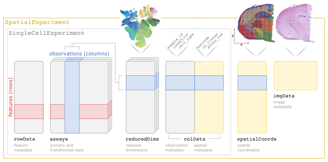Often, the starting point in spatial omics data analysis is a `r BiocStyle::Biocpkg('SpatialExperiment')` (or similar) object in `R` with Bioconductor. The data we consider here is a MERFISH assay of a mouse preoptic hypothalamus [@chenSpatiallyResolvedHighly2015; @moffittMolecularSpatialFunctional2018].```{r}#| label: load packagessuppressPackageStartupMessages({library(SpatialExperiment)library(spatstat.geom)library(spatstat.explore)library(dplyr)library(ggplot2)library(patchwork)library(reshape2)library(stringr)library(tidyr)library(magrittr)})``````{r, message=FALSE, warning=FALSE}#| label: load-data# source some helper functionssource("../code/utils.R")library('spatialFDA')theme_set(theme_light())# load the SpatialExperiment objectspe <-readRDS("../data/spe.rds")spe``````{r}colData(spe)$x <-spatialCoords(spe)[,'x']colData(spe)$y <-spatialCoords(spe)[,'y']annd <- zellkonverter::SCE2AnnData(spe)```We see that we have an object of class `r BiocStyle::Biocpkg('SpatialExperiment')` with $161$ genes (rows) and $73655$ cells. This object is very similar to a `r BiocStyle::Biocpkg('SingleCellExperiment')` object except it has the added `spatialCoords` slot. One slot in the `colData` is called `sample_id` which defines the so called z-slices. The three dimensional tissue is cut in the z-axis into consecutive two dimensional slices [@righelliSpatialExperimentInfrastructureSpatiallyresolved2022].Next, we want to extract three slices of this `r BiocStyle::Biocpkg('SpatialExperiment')` object and convert the 2D slices into `ppp` objects.```{r}# define the Z-stacks that you want to comparezstack_list <-list("-0.09", "0.01", "0.21")# small helper function to extract the z-slices and# convert them to `ppp` objectsselectZstacks <-function(zstack, spe) { spe[, spe$sample_id == zstack] |>.ppp(marks ="cluster_id")}pp_ls <-lapply(zstack_list, selectZstacks, spe) |>setNames(zstack_list)pp_ls```We see that we obtain a list of three `ppp` objects for the three z-slices $-0.09, 0.01, 0.21$.We can plot one of these slices, e.g. slice $-0.09$ with ggplot```{r}# create a dataframe from the point patternpp_df <- pp_ls[["-0.09"]] |>as.data.frame()# plot with ggplotggplot(pp_df, aes(x, y, colour = marks)) +geom_point(size =1) +coord_equal()```### WindowsAs stated above, one important aspect of a point pattern is the observation window. It represents the region in which a pattern is observed or e.g. a survey was conducted [@baddeleySpatialPointPatterns2015, pp. 85]. In most microscopy use cases we encounter window sampling. Window sampling describes the case where we don't observe the entire point pattern in a window but just a sample [@baddeleySpatialPointPatterns2015, pp. 143-145].The window of a point pattern does not need to be rectangular; we can receive round biopsies or calculate convex and non-convex hulls around our sample [@baddeleySpatialPointPatterns2015, pp. 143-145].Let's investigate the observation window for the slice $-0.09$.```{r, fig.width=10, fig.height=10}# subset point pattern listpp_sub <- pp_ls[["-0.09"]]# base R plot of all markspp_sub |>plot()```Here, we have a rectangular window around all points.Let's investigate what a round window would look like:```{r, fig.width=10, fig.height=10}pp_sub_round <- pp_sub# calculate circle with radius 850 µm and a center at the # centroid of the window would look likew <-disc(r =850, centroid.owin(Window(pp_sub)))Window(pp_sub_round) <- wpp_sub_round |>plot()```Correctly assigning windows is very important. The window should represent the space where points are expected. Point pattern methods assume that the process that we observe is a sample from a larger process (this concept is called window sampling). If the window is too small it would lead to a false underestimation of the area where the points can be potentially observed. This problem of where we can observe points and where not (beyond the boundary of the window) leads to a range of problems collectively called edge effects [@baddeleySpatialPointPatterns2015, pp. 143-145]. We will discuss these later.### MarksThe next concept that defines a point pattern is that marks can be associated with the points. The points can also have no mark, which we would call an unmarked point pattern```{r}unmark(pp_sub) |>plot()```Marks can be univariate or multivariate variables that are associated with the points [@baddeleySpatialPointPatterns2015, pp. 147]. In the context of cell biology we can distinguish between categorical marks (e.g. cell types) or continuous marks (e.g. gene expression).#### categorical MarksIn our example, we have a multitype point pattern, meaning there are different cell types that serve as marks for the point pattern. Multitype means that we consider all marks together. The opposite is multivariate, where we consider the marks independently [@baddeleySpatialPointPatterns2015, pp. 564 ff.].First the multitype case:```{r, fig.width=10, fig.height=10}pp_sub |>plot()```Then splitting the point pattern and plotting a multivariate view on the same pattern.```{r, fig.height=10, fig.width=10}pp_sub |>split() |>plot()```#### Continuous MarksMarks can as well be continuous as in the case of gene expression. We choose some genes from the original paper and look at their distribution [@baddeleySpatialPointPatterns2015 pp. 637; @moffittMolecularSpatialFunctional2018].```{r}# subset the original SpatialExperiment to our example slice -0.09sub <- spe[, spe$sample_id =="-0.09"]# Genes from Fig. 6 of Moffitt et al. (2018)genes <-c("Slc18a2", "Esr1", "Pgr")gex <-assay(sub)[genes, ] |>t() |>as.matrix() |>data.frame() |>set_rownames(NULL)# gene expression to marksmarks(pp_sub) <- gex```Now we have points with multivariate continuous marks:```{r, fig.height=5, fig.width=10}# create a dataframe in long format for plottingpp_df <- pp_sub |>as.data.frame() |>pivot_longer(cols =3:5)ggplot(pp_df, aes(x, y, colour =log(value +1))) +geom_point(size =0.5) +facet_wrap(~name) +coord_equal() +scale_color_continuous(type ="viridis")```We note that the expression of the genes `Pgr` and `Slc18a2` is very evenly distributed with some elevations in the middle of the structure. `Esr1` shows a half-circle like structure in expression. Note that the expression is here log transformed counts offset by one (to avoid problems with log of zero).#### Within Mark ComparisonWe can compare patterns between marks of the same type. This is referred to as a within mark comparison in our vignette. We can compare categorical marks, so the distribution of one single mark, e.g. a cell type.```{r, fig.height=5, fig.width=10}# create a dataframe from the point patternpp_df_categorical <-lapply(zstack_list, function(x) { df <- pp_ls[[x]] |>as.data.frame() df$stack <- xreturn(df)}) |>bind_rows()# select OD Mature cellspp_df_odmature <- pp_df_categorical[pp_df_categorical$marks =="OD Mature", ]ggplot(pp_df_odmature, aes(x, y, colour = marks)) +geom_point(size =0.5) +facet_wrap(~stack, scales ="free") +theme(aspect.ratio =1)```Here, we plot the distribution of mature oligodendrocytes across three slices of one 3D brain sample.Continuous marks can be compared as well, e.g. the expression of a gene across slices of a tissue```{r, fig.height=5, fig.width=10}pp_df <-lapply(zstack_list, function(x) {# subset the original SpatialExperiment to our example slice -0.09 sub <- spe[, spe$sample_id == x]# Genes from Fig. 6 of Moffitt et al. (2018) genes <-c("Slc18a2", "Esr1", "Pgr") gex <-assay(sub)[genes, ] |>t() |>as.matrix() |>data.frame() |>set_rownames(NULL)# gene expression to marksmarks(pp_ls[[x]]) <- gex df <- pp_ls[[x]] |>as.data.frame() df$stack <- xreturn(df)}) |>bind_rows()ggplot(pp_df, aes(x, y, colour =log(Esr1 +1))) +geom_point(size =0.5) +facet_wrap(~stack, scales ="free") +theme(aspect.ratio =1) +scale_color_continuous(type ="viridis")```We note that the expression of gene `Esr1` is differentially distributed across the slices of the 3D sample.#### CorrelationCorrelation is a second order quantity that measures the dependence between points [@baddeleySpatialPointPatterns2015 pp. 199]. A famous way to measure this is with Ripley's $K$, which is a cumulative function that quantifies the "number of $r$-neighbours of a typical random point" [@baddeleySpatialPointPatterns2015, pp. 204; @ripleySecondOrderAnalysisStationary1976].##### Global MeasuresGlobal correlation measures quantify the correlation in the entire window. Global Ripley's $K$ is defined as:$$\hat{K}(r) = \frac{|W|}{n(n-1)}\sum_{i=1}^n\sum_{j=1 \\j \neq i}^n\{d_{ij}\leq r\} e_{ij}(r)$$In the formula above we note a few things:- The function is normalised by the number of points $n$ and the window size $|W|$- the factor $e_{ij}(r)$ is an edge correction - see the section on `border corrections` further down in the vignette [@baddeleySpatialPointPatterns2015, pp. 204].Ripley's $K$ function can be variance stabilised, which is referred to as Besag's $L$ [@caneteSpicyRSpatialAnalysis2022; @besag1977contribution]. The idea behind variance stabilisation is to "uncouple" the relationship between mean and variance. By taking the square root of the function in question, the variance is nearly constant across the function [@bartlettUseTransformations1947].$$L(r) = \sqrt{\frac{K(r)}{\pi}}$$```{r, message = FALSE, warning=FALSE, fig.height=5, fig.width=10, results='hide'}res_ls <-lapply(list('Kest', 'Lest'), function(fun) { res <-calcMetricPerFov( spe,'OD Mature',subsetby ='sample_id',fun = fun,marks ='cluster_id',rSeq =NULL,by =c('Animal_ID', 'sample_id') ) res <-subset(res, sample_id %in%c('-0.09', '0.01', '0.21'))return(res)})p_ls <-lapply(res_ls, function(res) {plotMetricPerFov( res,theo =TRUE,correction ="iso",x ="r",imageId ='sample_id',legend.position ="right" )})``````{r, fig.height=5, fig.width=10}wrap_plots(p_ls, guides ='collect')```The strongest estimate of association between oligodendrocytes is found for the slices $0.01$. Slice $0.21$ does not show such a high degree of association at radii $\leq300$ as the other two slices. This means that the apparent clustering we see in the distribution of points is mainly due to an overall higher number of cells in slice $0.21$ and not a higher degree of association per se. The black line indicates the expected $K$ respectively $L$ function for a completely spatially random poisson process [@baddeleySpatialPointPatterns2015, pp. 132 ff.].Same can be done for the arrangement of `Microglia` cells across these three sections.```{r, eval=TRUE}res <-calcMetricPerFov( spe,'Microglia',subsetby ='sample_id',fun ='Lest',marks ='cluster_id',rSeq =NULL,by =c('Animal_ID', 'sample_id'))res <-subset(res, sample_id %in%c('-0.09', '0.01', '0.21'))plotMetricPerFov( res,theo =TRUE,correction ="iso",x ="r",imageId ='sample_id',legend.position ="right")```We note that the Microglia cells are distributed close to a Poisson Process across the different slices.A similar analysis can be performed for continuous marks. We calculate a mark weighted correlation function `markcorr`. The mark weighted correlation function is defined as:$$k_f(r) = \frac{\mathbb{E}[f(m(u),m(v))|u,v \in X]}{\mathbb{E}[f(M,M')]}$$where the numerator is the conditional expectation of the marks at location $u,v$ separated by a radius $r$ and $f$ can be any function linking the two marks. The denominator is the expectation of two random marks $M,M'$ [@baddeleySpatialPointPatterns2015, pp. 603].```{r}res <-calcMetricPerFov( spe,selection ='Esr1',subsetby ='sample_id',fun ='markcorr',marks ='Esr1',rSeq =NULL,by =c('Animal_ID', 'sample_id'),continuous =TRUE)res <-subset(res, sample_id %in%c('-0.09', '0.01', '0.21'))p <-plotMetricPerFov( res,correction ="iso",theo =TRUE,x ="r",imageId ='sample_id',legend.position ="right")p```We note that at very small radii the expression of the gene `Esr1` shows a high association with itself. Later on, the association is less pronounced than in the slices $-0.09$ and $0.01$.##### Local MeasuresNext to observation window metrics, we can calculate point level statistics as well. One such option is the local indicators of spatial association (LISA). This gives one curve per point in the field of view [@baddeleySpatialPointPatterns2015 pp. 247-248; @anselinLocalIndicatorsSpatial1995].```{r, message = FALSE, warning=FALSE, fig.height=5, fig.width=10, results='hide'}pp <-subset(pp_ls[["0.01"]], marks %in%"OD Mature")L_odmature_lisa <-localL(pp)df <-as.data.frame(L_odmature_lisa)dfm <- reshape2::melt(df, "r")get_sel <- dfm |> dplyr::filter(r >200.5630& r <201.4388, variable !="theo") |> dplyr::mutate(sel = value) |> dplyr::select(variable, sel)dfm <- dfm |>left_join(get_sel)p <-ggplot(dfm, aes(x = r,y = value,group = variable,colour = sel)) +geom_line(linewidth =1) +scale_color_continuous(type ="viridis") +geom_vline(xintercept =200) +theme(legend.position ="none") +ggtitle("LISA curves of slice 0.01")``````{r, fig.height=5, fig.width=10}p```These curves could be analysed using tools from functional data analysis such as functional PCA [@baddeleySpatialPointPatterns2015 pp. 247-248; @ramsayPrincipalComponentsAnalysis2005].### Cross Mark ComparisonThe same analyses as above can be performed between two cell types. The corresponding functions are called cross functions [@baddeleySpatialPointPatterns2015 pp. 594 ff.]. We implement (similar to the analyses above) a cross comparison between two cell types of interest. The provided functions enable this by giving a function and a vector with two cell types as input.```{r, message = FALSE, warning=FALSE, fig.height=5, fig.width=10}# select OD Mature and Microglia cellspp_df_odmature_microglia <- pp_df_categorical[pp_df_categorical$marks %in%c("OD Mature", "Microglia"), ]ggplot(pp_df_odmature_microglia, aes(x, y, colour = marks)) +geom_point(size =0.5) +facet_wrap( ~ stack, scales ="free") +theme(aspect.ratio =1)``````{r, message = FALSE, warning=FALSE, fig.height=5, fig.width=10, results='hide'}res <-calcMetricPerFov( spe,c("OD Mature", "Microglia"),subsetby ='sample_id',fun ='Lcross',marks ='cluster_id',rSeq =NULL,by =c('Animal_ID', 'sample_id'))res <-subset(res, sample_id %in%c('-0.09', '0.01', '0.21'))p <-plotMetricPerFov( res,theo =TRUE,correction ="iso",x ="r",imageId ='sample_id',legend.position ="right")``````{r, fig.height=5, fig.width=10}p```We note that there is not a very strong co-localisation indicated by the $L$ curves between mature oligodendrocytes and microglia cells. If we look at their spatial distribution that makes sense since microglia cells are distributed more or less homogeneously in the respective slices.### Edge effects and their corrections for spatial metricsEdge effects describe the phenomenon that not the entire point process is observed, but rather only the part within the window $W$. This means the value of various statistics could be biased along the edges [@baddeleySpatialPointPatterns2015, pp. 213].There are many corrections for edge effects that are briefly listed here [@baddeleySpatialPointPatterns2015, pp. 214-219]:Border correction:- In border correction the summation of data points is restricted to $x_i$ for which $b(x_i,r)$ is completely in the window $W$.Isotropic correction:- We can regard edge effect as a sampling bias. Larger distances (e.g. close to the edges) are less likely to be observed. This can be corrected for.Translation correction:- A stationary point process $X$ is invariant to translations. So the entire point process can be shifted by a vector $s$ to be at the position $X+s$.## Summary and Considerations- Point patterns are realisations of a point process. In the analysis we make inferences about the point process.- A point process assumes stochasticity. Therefore, HTS-based approaches are not suitable for point pattern analysis.- There are global metrics for the comparison within a celltype or between celltypes.- There are corresponding metrics for single cells and their interactions.- Point pattern analysis allows for the analysis of continuous gene expression marks as well.# Appendix## Session info```{r}sessionInfo()``````{r, include = FALSE}# Define the directory and file pathsdir_path <-"../tests/"dir_path_out <-"../tests/out"# Check if the directory exists, and create it if it doesn'tif (!dir.exists(dir_path)) {dir.create(dir_path)dir.create(dir_path_out)}res |>write.csv("../tests/out/test-00-overview-pp-R.csv")```


